Machine Learning Primer for Clinicians–Part 11

Alexander Scarlat, MD is a physician and data scientist, board-certified in anesthesiology with a degree in computer sciences. He has a keen interest in machine learning applications in healthcare. He welcomes feedback on this series at drscarlat@gmail.com.

Previous articles:

• An Introduction to Machine Learning
• Supervised Learning
• Unsupervised Learning
• How to Properly Feed Data to a ML Model
• How Does a Machine Actually Learn?
• Artificial Neural Networks Exposed
• Controlling the Machine Learning Process
• Predict Hospital Mortality
• Predict Length of Stay
• Unsupervised Anomaly Detection in Antibiograms

Basics of Computer Vision

The best ML models in computer vision, as measured by various image classification competitions, are the deep-learning, convolutional neural networks. A convolutional NN (convnet) for image analysis usually has an input layer, several hidden layers, and one output layer — like a regular, densely or fully connected NN, we’ve met already in previous articles:

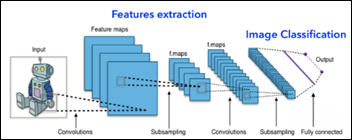
Modified from https://de.wikipedia.org/wiki/Convolutional_Neural_Network

The input layer of a convnet will accept a tensor in the form of:

• Image height
• Image width
• Number of channels: one if grayscale and three if colored (red, green, blue)

What we see as the digit 8 in grayscale, the computer sees as a 28 x 28 x 1 tensor, representing the intensity of the black color (0 to 255) at a specific location of a pixel:

From https://medium.com/@ageitgey/machine-learning-is-fun-part-3-deep-learning-and-convolutional-neural-networks-f40359318721

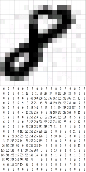
A color image would have three channels (RGB) and the input tensor would be image height x width x 3.

A convnet has two main parts: one that extracts features from an image and another, usually made of several fully connected NN layers, that classifies the features extracted and predicts an output — the image class. What is different from a regular NN and what makes a convnet so efficient in tasks involving vision perception are the layers responsible for the features extraction:

• Convolutional layers that learn local patterns of increasingly complex shapes
• Subsampling layers that downsize the feature map created by the convolutional layers while maximizing the presence of various features

Convolutional Layer

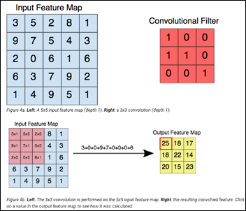
A convolutional layer moves a filter over an input feature map and summarizes the results in an output feature map:

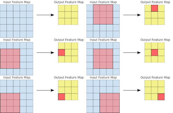
In the following example, the input feature map is a 5 x 5 x 1 tensor (which initially could have been the original image). The 3 x 3 convolutional filter is moved over the input feature map while creating the output feature map:

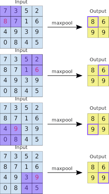
Subsampling Max Pool Layer

The input of the Max Pool subsampling layer is the output of the previous convolutional layer. Max pool layer output is a smaller tensor that maximizes the presence of certain learned features:

From https://developers.google.com/machine-learning/practica/image-classification/convolutional-neural-networks

Filters and Feature Maps

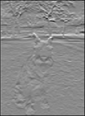
Original image:

A simple 2 x 2 filter such as 

[+1,+1]

[-1,-1] 

will detect horizontal lines in an image. The output feature map after applying the filter:

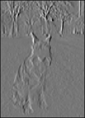
While a similar 2 x 2 filter 

[+1,-1]
[+1,-1] 

will detect vertical lines in the same image, as the following output feature map shows:

The filters of a convnet layer (like the simple filters used above for the horizontal and vertical line detection) are learned by the model during the training process. Here are the filters learned by a convnet first layer:

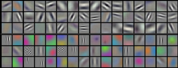
From https://www.amazon.com/Deep-Learning-Practitioners-Josh-Patterson/dp/1491914254

Local vs. Global Pattern Recognition

The main difference between a fully-connected NN we’ve met previously and a convnet, is that the fully connected NN learns global patterns, while a convnet learns local patterns in an image. This fact translates into the main advantages of a convnet over a regular NN with image analysis problems:

Spatial Hierarchy

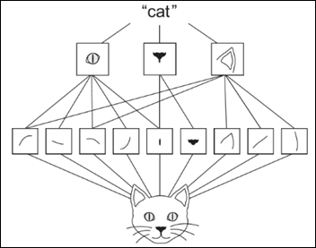
The first, deepest convolutional layers detect basic shapes and colors: horizontal, vertical, oblique lines, green spots, etc. The next convolutional layers detect more complex shapes such as curved lines, rectangles, circles, ellipses while the next layers identify the shape, texture and color of ears, eyes, noses, etc. The last layers may learn to identify higher abstract features, such as cat vs. dog facial characteristics – that can help with the final image classification. 

A convnet learns during the training phase the spatial hierarchy of local patterns in an image: 

From https://www.amazon.com/Deep-Learning-Python-Francois-Chollet/dp/1617294438

Translation and Position Invariant

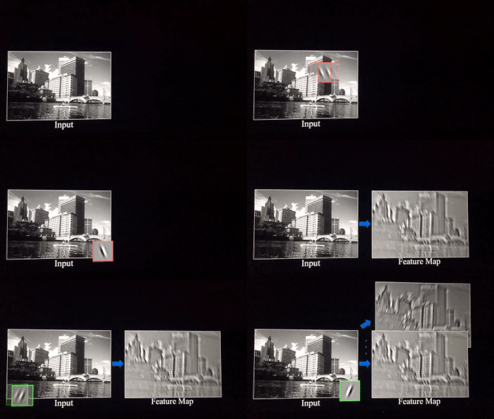
A convnet will identify a circle in the left lower corner of an image, even if during training the model was exposed only to circles appearing in the right upper corner of the images. Object or shape location within an image, zoom, angle, shear, etc. have almost no effect on a convnet capability to extract features from an image. 

In contrast, a fully-connected, dense NN will need to be trained on a sample for each possible object location, position, zoom, angle, etc. as it learns only global patterns from an image. A regular NN will require an extremely large number of (only slightly different) images for training.A convnet is more data efficient than a NN, as it needs a smaller number of samples to learn local patterns and features that in turn have more generalization power. 

The two filters below and their output feature maps — identifying oblique lines in an image. The convnet is invariant to the actual line position within the image. It will identify a local pattern disregarding its global location:

From https://ujjwalkarn.me/2016/08/11/intuitive-explanation-convnets/

Transfer Learning

Training a convnet on millions of labeled images necessitates powerful computers to work in parallel for many days and weeks. That’s usually cost prohibitive for most of us. Instead, one can use a pre-trained computer vision model that is available as open source. Keras (an open source ML framework) offers 10 such image analysis, pre-trained models.  All these models have been trained and tested on standard ImageNet databases. Their top, last layer has the same 1,000 categories: dogs, cats, planes, cars, etc. as this was the standardized challenge for the model.

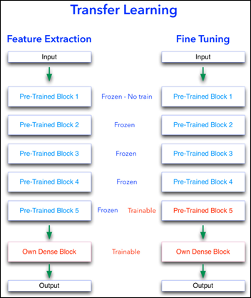
There are two main methods to perform a transfer learning and use this amazing wealth of image analysis experience accumulated by these pre-trained models:

Feature Extraction

1. Import a pre-trained model such as VGG16 without the top layer. The 1,000 categories of ImageNet standard challenge are most probably not well aligned with your goals.
2. Freeze the imported model so it will not be modified during training.
3. Add on top of the imported model, your own NN — usually a fully-connected, dense NN — that is trainable.

Fine Tuning

1. Import a pre-trained model without the top layer,
2. Freeze the model so it will not be modified during training, except …
3. Unfreeze the last block of layers of the imported model, so this block will be trainable.
4. Add on top of the imported model, your own NN, usually a dense NN.
5. Train the ML model with a slow learning rate. Large modifications to the original pre-trained model weights of its last block will practically destroy their “knowledge.”

Next Article

Identify Melanoma in Images