Machine Learning Primer for Clinicians–Part 9

Alexander Scarlat, MD is a physician and data scientist, board-certified in anesthesiology with a degree in computer sciences. He has a keen interest in machine learning applications in healthcare. He welcomes feedback on this series at drscarlat@gmail.com.

Previous articles:

• An Introduction to Machine Learning
• Supervised Learning
• Unsupervised Learning
• How to Properly Feed Data to a ML Model
• How Does a Machine Actually Learn?
• Artificial Neural Networks Exposed
• Controlling the Machine Learning Process
• Predict Hospital Mortality

Predict Length of Stay

In this article, we’ll walk through another end-to-end ML workflow while predicting the hospital LOS of ICU patients. The data is a subset of MIMIC3 – Multiparameter Intelligent Monitoring in Intensive Care – a de-identified, ICU, freely available database. Using a recipe detailed in my second book “Medical Information Extraction & Analysis: From Zero to Hero with a Bit of SQL and a Real-life Database,” I’ve summarized MIMIC3 into one table with 58,976 instances. Each row represents one admission. This table has the following columns, similar to the last article:

• Age, gender, admission type, admission source
• Daily average number of diagnoses
• Daily average number of procedures
• Daily average number of labs
• Daily average number of microbiology labs
• Daily average number of input and output events (any modification to an IV drip)
• Daily average number of prescriptions and orders
• Daily average number of  chart events
• Daily average number of procedural events (insertion of an arterial line)
• Daily average number of callouts for consultation
• Daily average number of notes (including nursing, MD notes, radiology reports)
• Daily average number of transfers between care units
• Total number of daily interactions between the patient and the hospital (a summary of all the above)

Using the daily averages of interactions allows the ML model to predict the LOS on a daily basis, as these averages are being modified on a daily basis.

I’ve removed mortality from this dataset as I don’t want to provide hints to the model in the form of mortality = short LOS. Besides, when asked to predict LOS, the model should not be aware of the overall admission outcome in terms of mortality as it may be considered data leaked from the future.

The hospital LOS in days is the label of the dataset, the outcome we’d like the ML model to predict in this supervised learning exercise. 

We will approach the LOS prediction challenge in two ways:

• Regression to arbitrary values – predict the actual number of days a specific admission is associated with
• Classification to several groups – predict to which class the admission belongs to (low, medium, high, very high LOS)

Short LOS Is Not Always a Good Outcome

Please keep in mind that a short LOS is not necessarily a good outcome. The patient may have died and thus a short LOS. In addition, there may be circumstances where a shorter LOS is accompanied by a higher readmission rate. In order to get the full picture, one needs to know the mortality and readmission rates associated with a specific LOS.

LOS – Regression

• Task: predict the number of days in hospital for an admission
• Experience: MIMIC3 subset detailed above
• Performance: Mean Absolute Error (MAE) between prediction and true LOS

The Python code used for predicting LOS with regression ML models, is publicly available at Kaggle.

Data was separated into a train (47,180 admissions) and test (11,796 admissions) datasets as previously explained.

I’ve trained and cross-evaluated 12 regressor models: Gradient Boosting Regressor, Extra Trees Regressor,  Random Forest Regressor,  Bayesian Ridge, Ridge, Kernel Ridge, Linear SVR, SVR, Elastic Net,  Lasso, SGD Regressor, Linear Regression. The best model, Random Forest Regressor (RFR), came on top with a Mean Absolute Error (MAE) of 1.45 days (normalized MAE of 11.8 percent). This performance was measured on the test subset, data the model has never seen during training.

The learning curves show that the model is overfitting, as the validation MAE is stuck on approximately 0.12 or 12 percent, while the error on the training set is much lower at 5 percent.Thus, the model would benefit from more samples, better feature engineering, or both.

Features Importance

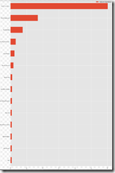
RFR offers a view into its decision-making process by showing the most important features related to LOS:

Note in the following sorted list of features that age is not an important predictor of LOS, relative to the other features. For example, the number of daily notes is about 10 times more important as a predictor than age, while the daily average number of transfers – the best LOS predictor – is approximately 85 times more important than age:

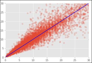
Below is the chart of the predicted vs. the true LOS on the test dataset. On the X axis are the number of real days in the hospital and the Y axis is the predicted LOS by the RFR model. In a perfect situation all points would fall on the blue identity line where X=Y.

Neural Network (NN)

I’ve trained and evaluated several NN on the above data set: from small 15,000 to 20 million weights in different combinations of dense layers and units (a.k.a. neurons).One of the NN’s (with 12.6 million trainable parameters) learning curves:

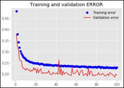
The best NN MAE is 2.39 days or a normalized MAE of 19.5 percent. The NN performance is worse when compared to the RFR model.

LOS – Classification

The Python code used for this part of the article, is publicly available at Kaggle.

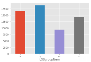
Using the same dataset as the one used for regression above, I’ve grouped the admissions into the following four classes:

1. Between 0 and 4 days LOS (group 0 in the chart below)
2. Between 4 and 8
3. Between 8 and 12
4. More than 12 days of LOS (group 3 below)

• Task: predict the LOS group from the four classes defined above (0,1,2,3)
• Experience: same MIMIC3 subset used above, with the daily averages of interactions between patient and hospital
• Performance: Accuracy, F1 score, ROC AUC as explained in the previous article

I’ve evaluated the following classifiers: Logistic Regression, Random Forest, Stochastic Gradient, K-Nearest Neighbors, Decision Tree, Support Vector Machine. The best classifier model came (again) the Random Forest Classifier (RFC) – an ensemble of weak predictors. Below is the RFC confusion matrix on the test dataset:

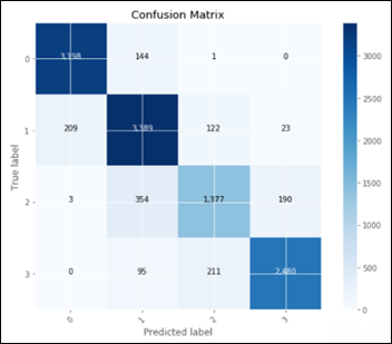
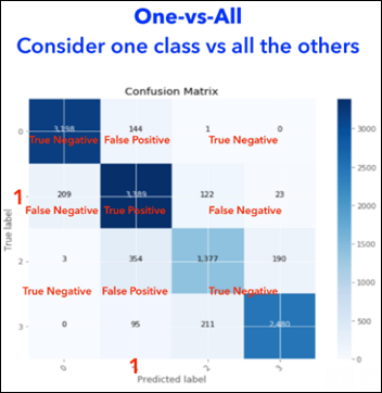
The above confusion matrix shows the predicted vs. true labels for all the 4 LOS groups.  We cannot use such a confusion matrix for calculating precision, recall, F1 and AUC as these metrics require a simpler, 2 X 2 confusion matrix with TP, FP, TN and FN. We need to calculate for each one of the four LOS groups – its own confusion matrix and derived metrics. 

Each one of these classes is going to be compared against all the other groups, thus the name of the technique one-vs.-all, so the results can be summarized in a 2 X 2 confusion matrix:

• TP = model predicted a class X and it was truly class X
• TN = model predicted it’s not class X and it was not X
• FP = model predicted it’s class X but it was not X
• FN = model predicted it is not class X, and it actually was X

In the following figure, we consider only one class, the second one, labeled 1 (as counting starts with 0) and calculate the confusion matrix of the model in regard to this class:

After we repeat the above exercise four times (as the number of classes), we end up with four confusion matrices, one for each class. We can now summarize these four confusion matrices and calculate the overall performance of the RFC model as well as compare the performance related to each one of the LOS groups:

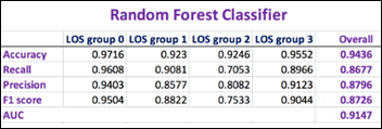
The higher the F1 score and AUC, the better is the model performance.

The best NN model (with approx. 12.6 million trainable parameters) performance in comparison:

Both the RFC and the NN models are performing best when evaluated on the first group-vs.-all: LOS below vs. above 4 days (LOS group 0).

Random Forest is an ensemble of other weak predictor models. Still it outperforms any NN by a large margin with both the regression and classification challenges of predicting the LOS. 

It is interesting and maybe worth an article by itself, how a group of under performing “students” manage to use their error diversity in achieving a better outcome than the best-in-class NN models.

Next Article

Unsupervised Anomaly Detection in Antibiotic Resistance Patterns