A Machine Learning Primer for Clinicians–Part 3

Alexander Scarlat, MD is a physician and data scientist, board-certified in anesthesiology with a degree in computer sciences. He has a keen interest in machine learning applications in healthcare. He welcomes feedback on this series at drscarlat@gmail.com.

Previous articles:

1. An Introduction to Machine Learning
2. Supervised Learning

Unsupervised Learning

In the previous article, we defined unsupervised machine learning as the type of algorithm used to draw inferences from input data without having a clue about the output expected. There are no labels such as patient outcome, diagnosis, LOS, etc. to provide a feedback mechanism during the model training process.

In this article, I’ll focus on the two most common models of unsupervised learning: clustering and anomaly detection.

Unsupervised Clustering

Note: do not confuse this with with classification, which is a supervised learning model introduced in the last article.

As a motivating factor, consider the following image from Wikipedia:

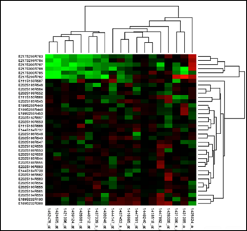
The above is a heat map that details the influence of a set of parameters on the expression (production) of a set of genes. Red means increased expression and green means reduced expression. A clustering model has organized the information in a heat map plus the hierarchical clustering on top and on the right sides of the diagram above. 

There are two types of clustering models:

• Models that need to be told a priori the number of groups / clusters we’re looking for
• Models that will find the optimal number of clusters

Consider a simple dataset:

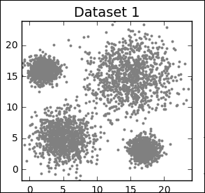
Problem definition:

• Task: identify the four clusters in Dataset1.
• Input: sets of X and Y and the number of groups (four in the above example).
• Performance metric: total sum of the squared distances of each point in a cluster from its centroid (the center of the cluster) location.

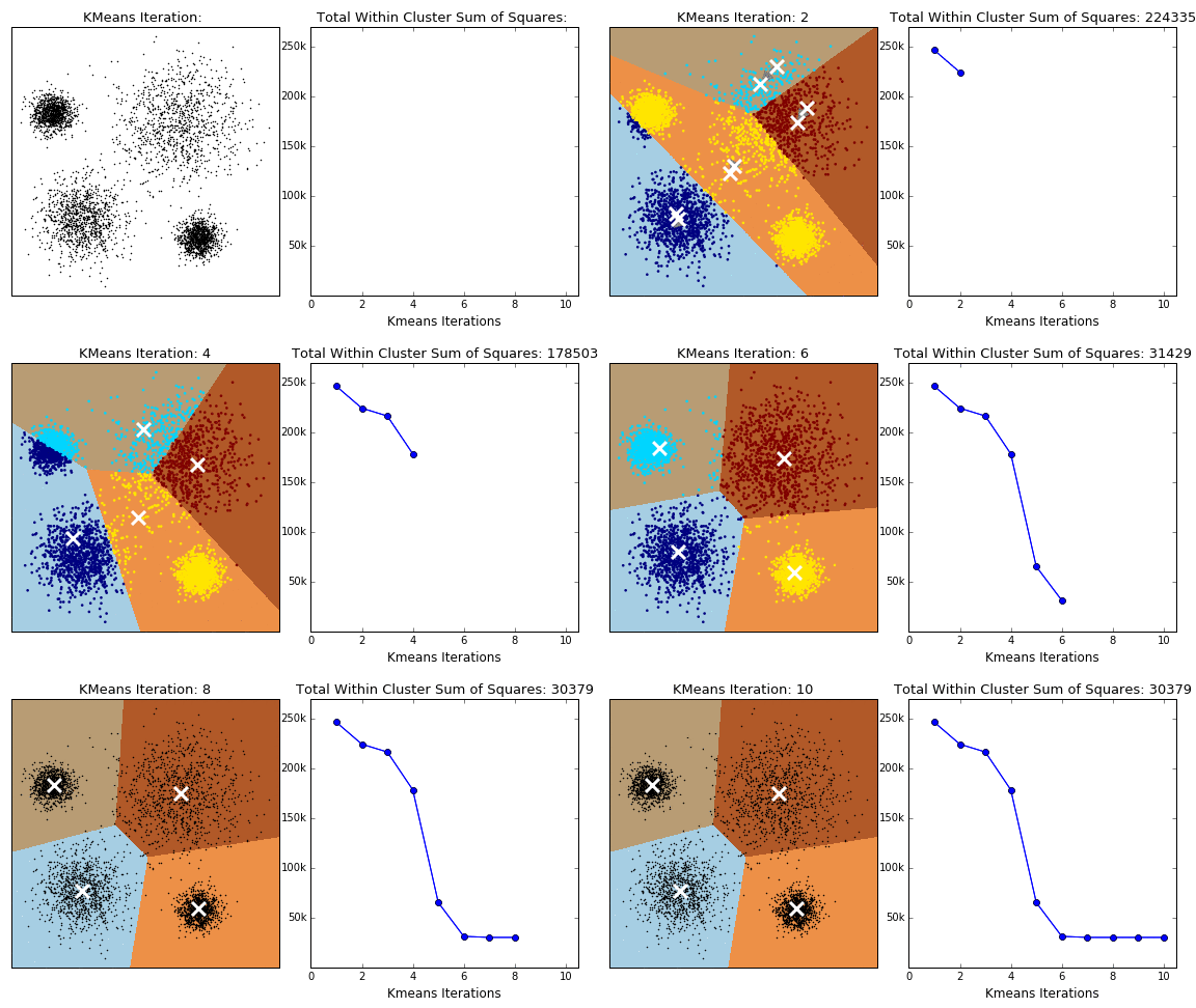
The model initializes four centroids, usually at a random location. The centroids are then moved according to a cost function that the model tries to minimize at each iteration. The cost function is the total sum of the squared distance of each point in the cluster from its centroid. The process is repeated iteratively until there is little or no improvement in the cost function.

In the animation below you can see how the centroids – white X’s – are moving towards the centers of their clusters in parallel to the decreasing cost function on the right.

While doing great on Dataset1, the same model fails miserably on Dataset2, so pick your clustering ML model wisely by exposing the model to diverse experiences / datasets:

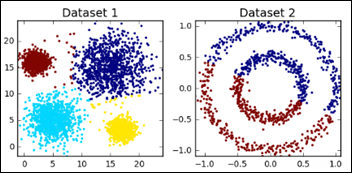
Clustering models that don’t need to know a priori the number of centroids (groups) will have the following problem definition:

• Task: identify the clusters in Dataset1 with the lowest cost function.
• Input: sets of X and Y (there are NO number of groups / centroids).
• Performance metric: same as above.

The model below initializes randomly many centroids and then works through an algorithm that tells it how to consolidate together other neighboring centroids to reduce the number of groups to the overall lowest cost function.

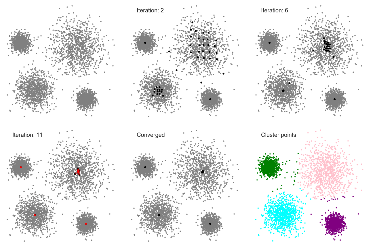
From “Clustering with SciKit” by David Sheehan

3D Clustering

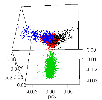
While the above example had as input two dimensions (features) X and Y, the following gene expression in a population has three dimensions: X, Y, and Z. The mission definition for such a clustering ML model is the same as above, except the input has now three features: X, Y, and Z.

The animated graphic is at www.arthrogenica.com

Unsupervised Anomaly Detection

As a motivating factor, consider the new criteria for early identification of patients at risk for sepsis or septic shock, qSOFA 2018. The three main rules:

• Glasgow Coma Scale (GCS) < 15
• Respiratory rate (RR) >= 22
• Systolic blood pressure (BP) <=100 mmHg

Let’s focus on two parameters, RR and BP, and a patient who presents with:

• RR = 21
• BP = 102

A rule-based engine with only two rules will miss this patient, as it doesn’t sound the alarm per the above qSOFA definition. Not if the rule was written with AND and not it had OR between the conditions. Can a ML model do better? Would you define the above two parameters, when taken together, as an anomaly ? 

Before I explain how a machine can detect anomalies unsupervised by humans, a quick reminder from Gauss (born 1777) about his eponymous distribution.

One-Variable Gaussian Distribution

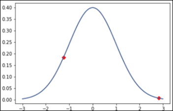
You may remember from statistics that the above bell-shaped normal Gaussian distribution can accurately describe many phenomena around us. The mean on the above X axis is zero and then there are several standard deviations around the mean (from -3 to +3). The Y axis defines the probability of X. Each point on the chart has a probability of occurrence: the red dot on the right can be defined as an anomaly with a probability of ~ 1 percent. The dot on the left side has a probability of ~ 18 percent,  so most probably it’s not an anomaly. 

The sum (integral) of a Gaussian probability distribution is one, or 100 percent. Thus even an event right on top of our chart has a probability of only 40 percent. Given a point on the X axis and using the Gaussian distribution, we can easily predict the probability of that event happening.

Two-Variable Gaussian Distribution

Back to the patient that exhibits RR = 21 and BP=102 and the decision whether this patient is in for a septic shock adventure or not. There are two variables: X and Y, and a new problem definition:

• Task: automatically identify instances as anomalies if they are beyond a given threshold. Let’s set the anomaly threshold at three percent.
• Input: sets of X and Y and the threshold to be considered an anomaly (three percent).
• Performance metric: number of correct vs. incorrect classifications with a test set, with known anomalies (more about unbalanced classes in next articles).

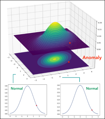
The following 3D peaks chart has X (RR), Y (BP), and the Gaussian probability as Z axis. Each point on the X-Y plane has a probability associated with it on the Z axis. Usually a peaks chart has an accompanying contour map  in which the 3D is flattened to 2D, with the color still expressing the probability.

Note the elongated, oblong shape of both the peaks chart and the contour map underneath it. This is the crucial fact: the shape of the Gaussian distribution of X and Y  is not a circle (which we may have naively assumed), it’s elliptical. On the peaks chart, there is a red dot with its corresponding red dot on the contour map below. The elliptic shape of our probability distribution of X and Y helps visualizing the following:

• Each parameter, when considered separately on its own probability distribution, is within its normal limits.
• Both parameters, when taken together, are definitely abnormal, an anomaly with a probability of ~ 0.8 percent (0.008 on the Z axis), much smaller than the three percent threshold wee set above.

Unsupervised anomaly detection should be considered when:

• The number of normal instances is much larger than the number of anomalies. We just don’t have enough samples of labeled anomalies to use with a supervised model.
• There may be unforeseen instances and combinations of parameters that when considered together are abnormal. Remember that a supervised model cannot predict or detect instances never seen during training. Unsupervised anomaly detection models can deal with the unforeseen circumstances by using a function from the 1800s.

Scale the above two-parameter model to one that considers hundreds to thousands of patient parameters, together and at the same time, and you have an unsupervised anomaly detection ML model to prevent patients deterioration while being monitored in a clinical environment. 

The fascinating part about ML algorithms is that we can easily scale a model to thousands of dimensions while having, at the same time, a severe human limitation to visualize more than 5D (see previous article on how a 4D / 5D problem may look).

Next Article

How to Properly Feed Data to a ML Model