A Machine Learning Primer for Clinicians–Part 5

Alexander Scarlat, MD is a physician and data scientist, board-certified in anesthesiology with a degree in computer sciences. He has a keen interest in machine learning applications in healthcare. He welcomes feedback on this series at drscarlat@gmail.com.

Previous articles:

1. An Introduction to Machine Learning
2. Supervised Learning
3. Unsupervised Learning
4. How to Properly Feed Data to a ML Model

How Does a Machine Actually Learn?

Most ML models will have the following components:

• Weights – units that contain the model parameters and are modified with each new learning experience. a.k.a train epoch.
• Metric – a measure (accuracy, mean square error) of the distance between the model prediction and the true value of that epoch.
• Loss or Cost Function – used to update the weights with each train epoch according to the calculated metric.
• Optimizer – algorithm overseeing the loss function so the model will find the global minimum in a reasonable time frame, basically preventing the model from wondering all over the loss function hyperspace.

The learning process or model training is done in epochs. With each epoch, the model is exposed to a batch of samples. 

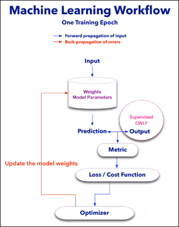
Each epoch has two steps:

1. Forward propagation of the input. The input features undergo math calculations with all the model weights and the model predicts an output.
2. Back propagation of the errors. The model prediction is compared to the real output. This metric is used by the loss function and its master – the optimizer algorithm – to update all the weights according to the last epoch performance.

Consider a model, in this case a neural network (NN) that tries to predict LOS using two features: age and BMI. We have a table with 100 samples / instances / rows and three columns: age, BMI, and LOS.

• Task: using age and BMI, predict the LOS.
• Input: age and BMI,
• Output: LOS.
• Performance: mean square error (MSE),  the squared difference between predicted and true value of LOS.

Forward Propagation of the Input

Input is being fed one batch at a time. In our example, let’s assume the batch size is equal to one sample (instance).

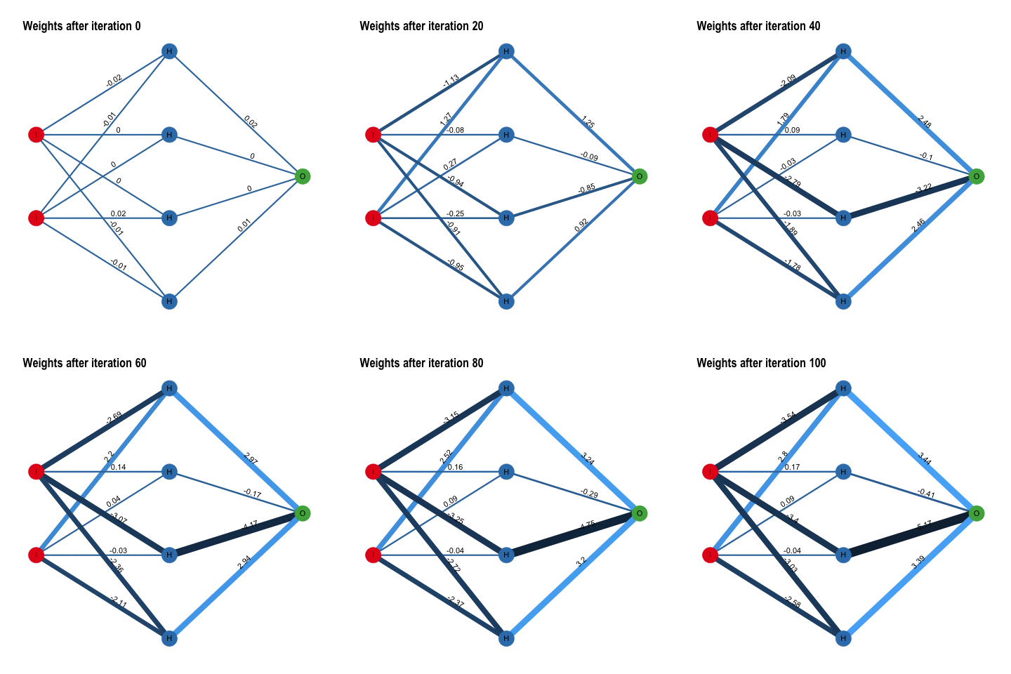
In the above case, one instance enters the model at the two left red dots: one for age and one for BMI (I stands for Input). The model weights are initialized as very small, random numbers near zero.

All the input features of one instance interact simultaneously through a complex mathematical transformation with all the model parameters (weights are denoted with H from hidden). These interactions are then summarized as the model LOS prediction at the rightmost green dot – output.

Note the numbers on the diagram above and the color of the lines as weights are being modified according to the last train epoch performance. Blue = positive feedback vs. black = negative feedback.

The predicted value of LOS will be far off initially as the weights have been randomly initialized, but the model improves iteratively as it is exposed to more experiences. The difference between the predicted and true value is calculated as the model metric.

Back Propagation of the Error

The model optimizer updates all the weights simultaneously, according to the last metric and loss function results. The weights are slightly modified with each sample the model sees – the cost function is providing the necessary feedback from the metric that measures the distance between the recent prediction vs. the true LOS value. The optimizer basically searches for the global minimum of the loss function

This process is now repeated with the next instance (sample or batch) and so on. The model learns with each and every experience until it is trained on the whole dataset.

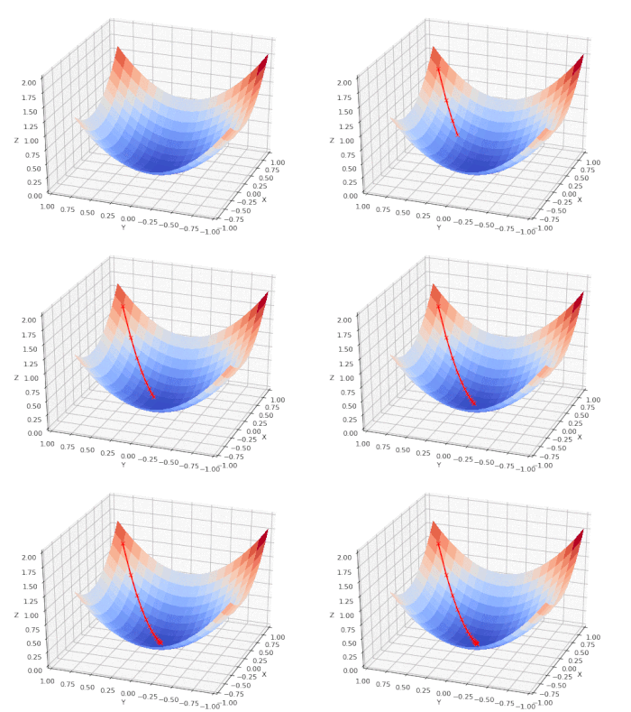
The cost function below shows how the model approaches the minimum with each iteration / epoch.

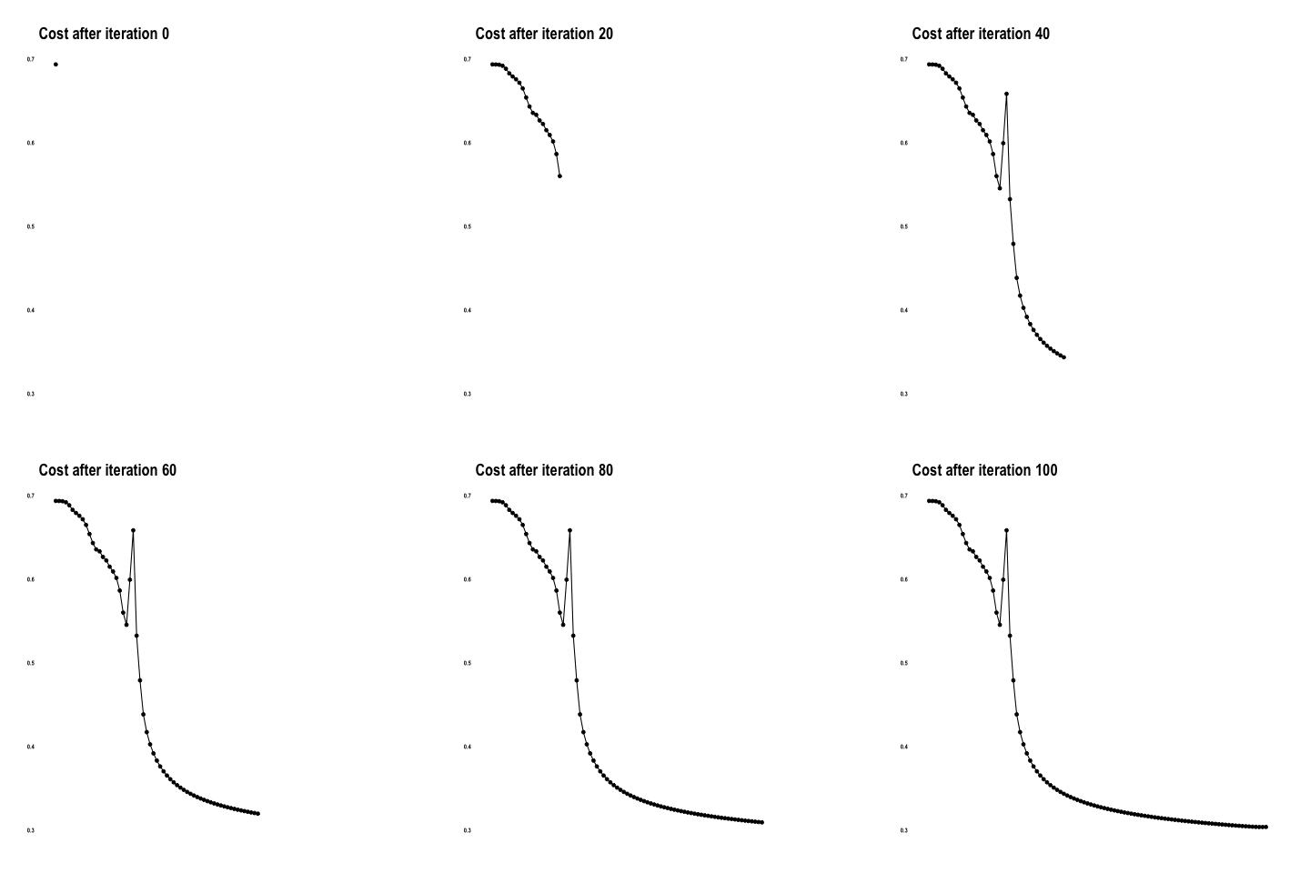
From “Coding with Data” by Tamas Szilagyi.

Once the training has ended, the model has a set of weights that have been exposed to 100 samples of age and BMI. These weights have been iteratively modified during the forward propagation of the input and the back propagation of errors. Now, when faced with a new, never before seen instance of age and BMI, the model can predict the LOS based on previous experiences.

Unsupervised Learning

Just because there is no output (labels) in unsupervised learning doesn’t mean the model is not constrained by a loss / cost function. In the clustering algorithm from the article on Unsupervised Learning , for example, its cost function was the distance between each point and its cluster centroid, and the model optimizer tried to minimize this function with each iteration.

Loss / Cost Function vs. Features

We can chart the loss function (Z) vs. the input features: age (X) and BMI (Y) and follow the model as it performs a gradient descent on a nice, convex cost function that has only one (global) minimum:

Sometimes two features can present a more complex landscape of a loss function, one with many local minima, saddles and the one, much sought after, global minimum:

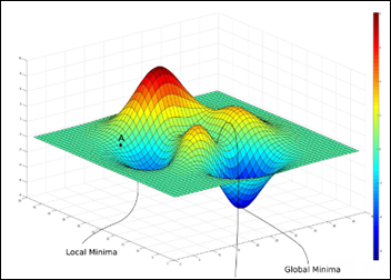
From “Intro to optimization in deep learning” – PaperSpace Blog.

Here is a comparison of several ML model optimizers, competing to escape a saddle point on a loss function, in order to get to the optimizers’ nirvana – the global minimum. Some optimizers are using a technique called momentum, which simulates a ball accumulating physical momentum as it goes down hill.  Getting stuck on a saddle in hyperspace is not a good thing for a model / optimizer, as the poor red Stochastic Gradient Descent (SGD) optimizer may be able to tell, if it will ever escape.

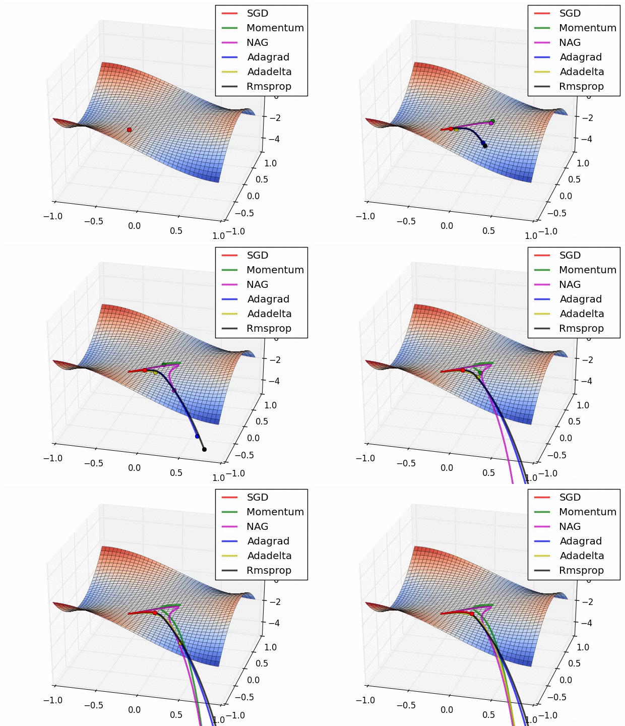
From “Behavior of adaptive learning rate algorithms at a saddle point” – NVIDIA blog.

Just to give you an idea of how complex a loss / cost function landscape can be, below is the loss function of VGG-56 – a known image analysis model trained on a set of several million images. This specific model loss function has as X – Y axes the two main principal components of all the features of an image. Z axis is the cost function.

The interesting landscape below is where VGG-56 has to navigate and find the global minimum – not just any minimum, but the lowest of them. Not a trivial task.

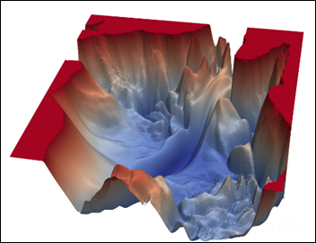
From “Intro to optimization in deep learning” – PaperSpace Blog.

Compressing many dimensions an image usually has, into only two (X-Y) – while minimizing the loss of variance – is usually a job performed by principal component analysis (PCA),  a type of unsupervised ML algorithm. That’s another aspect of ML – models that can help us visualize stuff which was unimaginable only a couple of years ago, such as the 3D map of the cost function of an image analysis algorithm.

Next Article

Artificial Neural Networks Exposed