Machine Learning Primer for Clinicians–Part 8

Alexander Scarlat, MD is a physician and data scientist, board-certified in anesthesiology with a degree in computer sciences. He has a keen interest in machine learning applications in healthcare. He welcomes feedback on this series at drscarlat@gmail.com.

Previous articles:

• An Introduction to Machine Learning
• Supervised Learning
• Unsupervised Learning
• How to Properly Feed Data to a ML Model
• How Does a Machine Actually Learn?
• Artificial Neural Networks Exposed
• Controlling the Machine Learning Process

Predict Hospital Mortality

In this article, we’ll walk through our first end-to-end ML workflow while predicting the hospital mortality of ICU patients.

The Python code I’ve used for this article, is publicly available at Kaggle. The data for this exercise is a subset of MIMIC3 (Multiparameter Intelligent Monitoring in Intensive Care), a de-identified, freely available ICU database. MIMIC3 is a RDBMS (relational database management system) with many tables, relationships, and information on 59,000 admissions.

Since no ML model can digest data in a relational format, the first step is to decide how to flatten the relational structure so that each instance will represent one admission.

Hypothesis on the Number of Patient-Hospital Interactions

One can learn a lot about the patient’s outcome from the number of interactions a patient has with the hospital: number of labs, orders, meds, imaging reports, etc. Not necessarily the quality of these interactions (abnormal or normal, degree of abnormality, etc.), just their numbers. It is of course, an oversimplification of the patient outcome prediction problem, but it is an easier toy-model to explain compared to a full-blown, production-ready model.  

We’ll present the ML model with the daily average of interactions, such as the daily average number of labs, meds, consultations, etc. In real life with this arrangement, the ML model can predict mortality each and every day as the average number of interactions between patient and hospital changes daily. 

Flatten MIMIC Into a Table

Using a method detailed in my second book “Medical Information Extraction & Analysis: From Zero to Hero with a Bit of SQL and a Real-life Database,” I’ve summarized MIMIC3 into one table with 58,976 instances. Each row represents one admission. This table has the following columns:

• Age, gender, admission type, admission source
• Daily average number of diagnoses
• Daily average number of procedures
• Daily average number of labs
• Daily average number of microbiology labs
• Daily average number of input and output events (any modification to an IV drip)
• Daily average number of prescriptions and orders
• Daily average number of  chart events
• Daily average number of procedural events (insertion of an arterial line)
• Daily average number of callouts for consultation
• Daily average number of notes (including nursing, MD notes, radiology reports)
• Daily average number of transfers between care units
• Total number of daily interactions between the patient and the hospital (a summary of all the above)

The hospital mortality is the label of the set, the outcome we’d like the ML model to predict in this supervised learning, binary classification exercise.

Prepare the Data

As previously detailed, I’ve imputed the missing values with the average, the most frequent value, or just “NA.”

Summary of some basic stats:

Leaking Data from the Future

LOS was eliminated from the dataset as it is never a good idea to provide the model information from the future. When asked to predict mortality, the LOS is not yet known, so it should not be given to the model during training. Leaking data to the ML model is equivalent to cheating yourself — the model will have a stellar performance in the lab and a terrible one in real life.

Skewed Data and Normalization

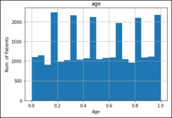
Histogram of age and the number of patients in each category:

The raw data in the above chart is skewed. There are newborns but no other pediatric patients in MIMIC3. There’s also a sharp cut-off at the age of 90. This is partially corrected during the normalization process. The same parameter of age  after normalization:

The process of normalization was applied to all the features.

Mortality and Imbalanced Datasets

The in-hospital mortality of the patients in MIMIC3 dataset is 5,855 / 58,967 = 9.93 percent  of admissions.

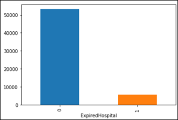
This is considered an imbalanced dataset as the classes of lived vs. expired are imbalanced 9:1. Consider a simple, dumb model, one that always predicts that the patient lives and it assumes 0 percent mortality.

Accuracy is defined as (true positives + true negatives) / all samples, so this model has a fantastic accuracy of 90 percent on MIMIC3 dataset. With 100 patients and a model predicting that all patients lived, TN=90 and FN=10, the accuracy is (0+90)/100=90 percent.

If you need more confusion about TP, FP, TN, FN, and their derivatives, please explore the fascinating confusion matrix.

This exercise with a dumb model provides the necessary perspective on the problem, as it gives us a certain baseline to compare against the machine. We know by now that a 90 percent accuracy is not such a high goal to achieve. It’s considered common sense in ML to try come up with a sanity check, a baseline against which to compare a metric, before we measure the machine performance on a task. 

When a problem involves a moderate to highly imbalanced classes situation == such as mortality in our dataset being 10 percent — accuracy is not the only metric to monitor, as it may be quite misleading. The relevance of the predictions is an important parameter as well:

Precision = TP/(TP+FN)

How many selected items were relevant? Our dumb model’s precision is 0, as no true positives (TP) have been selected (0/0+10).

Recall = TP/TP+FP

How many relevant items are selected?  Recall for this model is also 0, as nothing predicted was relevant (actually recall is indeterminate 0/0).

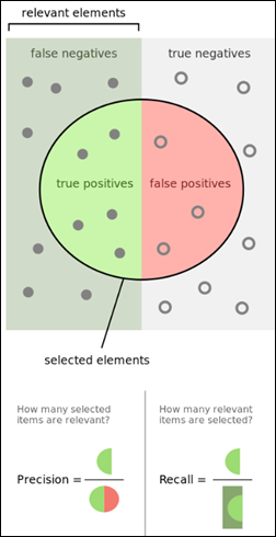
From Wikipedia.

One Metric Only

A ML model needs one, and only one, metric to use for calculations of the loss function and optimizer. The model will refuse to work if presented with two metrics, such as precision and recall. In the case of imbalanced classes, precision and recall have one prodigy, named F1 score — the harmonic mean of precision and recall. A higher F1 score is better.

In the following examples, I’ve used accuracy, precision, recall and F1 score as the models’ metrics for optimization, but only one metric at a time. In addition, I’ve also optimized the models on the area under the vurve (AUC) of the receiver operating characteristic (ROC), even though ROC AUC is best used with balanced classes. A higher AUC is better.

Task: predict mortality as a supervised learning classification based on a binary decision (yes / no)
Experience: MIMIC3 subset detailed above
Performance: accuracy, F1 score, and ROC AUC 

The original dataset was split into two subsets as previously explained:

Training: 47,180 instances or samples (admissions)
Testing: 11,796 instances

Models

Initially I’ve trained and cross-evaluated seven classifier models: logistic regression, random forest, stochastic gradient descent, K-nearest neighbors, decision tree, Gaussian naive Bayes, support vector machine. These models have used the various metrics detailed above for their optimization algorithms, one metric at a time.

The best model came as random forest classifier with the following learning curves while optimizing on ROC AUC:

The confusion matrix for the random forest classifier (RF) model on the test subset of 11,796 samples, never seen before by the RF model:

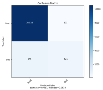
• TN: 10528
• FP: 101
• FN: 646
• TP: 521

The above confusion matrix translates into the following performance metrics for the RF model:

• Accuracy 93.7 percent
• Precision 83.9 percent
• Recall 44.4 percent
• F1 score 0.581
• AUC 0.717

Feature Importance

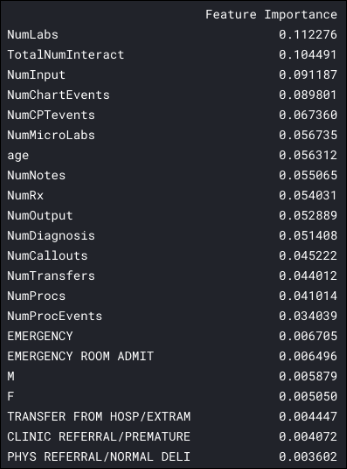
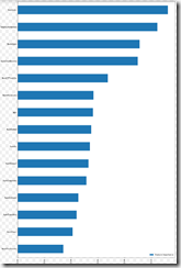
We can ask the RF model to display the most important features in the data that helped the algorithm in the decision making process about hospital mortality:

The daily average number of labs seems to be the most important feature for this ML model, almost twice more important than the age parameter.

Note that six features are more important in predicting the admission mortality than the patient’s age:

I’ve tested several neural network architectures and the best results came from a NN with three layers fully interconnected (dense) of 2,048 units each. 

The output sigmoid unit produces a probability between 0 and 1. If this last unit output is above 0.5, the ML model will predict that the patient died. If the output is below 0.5, the model will predict that the patient lived.

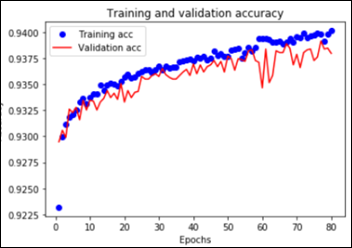
Overall the NN had 8.4 million trainable parameters. In order to prevent overfitting, I’ve employed dropout and regularizers with a relatively slow learning rate, as explained in article #7 in this series. The NN training and validation learning curves showing model overfitting after approximately 55 epochs:

The confusion matrix for the above NN model on the test subset of 11,796 samples, never seen before by the model:

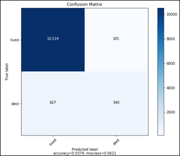
• TN: 10524
• FP: 105
• FN: 627
• TP: 540

The above confusion matrix translates into the following performance metrics for the RF model:

• Accuracy 93.8 percent
• Precision 83.7 percent
• Recall 46.3 percent
• F1 score 0.596
• AUC 0.726

A comparison between RF and NN performances on the prediction of hospital mortality:

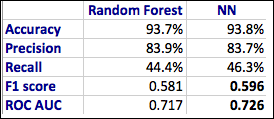
Next time you are impressed by a high accuracy of a prediction made by a ML model, remember that high accuracy may be accompanied by very low precision and recall, especially with problems where the data classes are imbalanced. In such cases, politely ask for the additional metrics: confusion matrix, Precision, Recall, F1 score, and AUC. 

As a sanity check, always try to estimate what a No-ML-No-AI kind of model would have predicted in the same situation. Use this estimate as the first baseline to test your ML model against.

Next Article

Predict Hospital Length of Stay