A Machine Learning Primer for Clinicians–Part 2
Alexander Scarlat, MD is a physician and data scientist, board-certified in anesthesiology with a degree in computer sciences. He has a keen interest in machine learning applications in healthcare. He welcomes feedback on this series at drscarlat@gmail.com.

To recap from Part 1, the difference between traditional statistical models and ML models is their approach to a problem:

We feed Statistics as an Input and some Rules. It provides an Output.
With a ML model, we have two steps:
- We feed ML an Input and the Output and the ML model learns the Rules. This learning phase is also called training or model fit.
- Then ML uses these rule to predict the Output.
In an increasing number of fields, we realize that these rules learned by the machine are much better than the rules we humans can come up with.
Supervised vs. Unsupervised Learning
With the above in mind, the difference between supervised and unsupervised is simple.
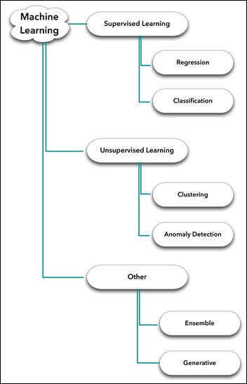
- Supervised learning. We know the labels of each input instance. We have the Output (discharged home, $85,300 cost to patient, 12 days in ICU, 18 percent chance of being readmitted within 30 days). Regression to a continuous variable (number) and Classification to two or more classes are the main subcategories of supervised learning.
- Unsupervised learning. We do not have the Output. Actually, we may have no idea what the Output even looks like. Note that in this case there’s no teacher (in the form of Output) and no rules around to tell the ML model what’s correct and what’s not correct during learning. Clustering, Anomaly Detection, and Primary Component Analysis are the main subcategories of unsupervised learning.
- Other. Models working in parallel, one on top of another in ensembles, some models supervising other models which in turn are unsupervised, some of these models getting into a “generative adversarial relationship” with other models (not my terminology). A veritable zoo, an exciting ecosystem of ML model architectures that is growing fast as people experiment with new ideas and existing tools.
Supervised Learning – Regression
With regression problems, the Output is continuous — a number such the LOS (number of hours or days the patient was in hospital) or the number of days in ICU, cost to patient, days until next readmission, etc. It is also called regression to continuous arbitrary values.
Let’s take a quick look at the Input (a thorough discussion about how to properly feed data to a baby ML model will follow in one of the next articles).
At this stage, think about the Input as a table. Rows are samples and columns are features.
If we have a single column or feature called Age and the output label is LOS, then it may be either a linear regression or a polynomial (non-linear) regression.
Linear Regression
Reusing Tom Mitchell definition of a machine learning algorithm:
” A computer program is said to learn from Experience (E) with respect to some class of tasks (T) and performance (P) – IF its performance at tasks in T, as measure by P, improves with experience (E)”
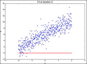
- The Task is to find the best straight line between the scatter points below – LOS vs. age – so that, in turn, can be used later for prediction of new instances.
- The Experience is all the X and Y data points we have.
- The Performance will be measured as the distance between the model prediction and the real value.
The X axis is age, the Y axis is LOS (disregard the scale for the sake of discussion):
Monitoring the model learning process, we can see how it approaches the best line with the given data (X and Y) while going through an iterative process. This process will be detailed later in this series:
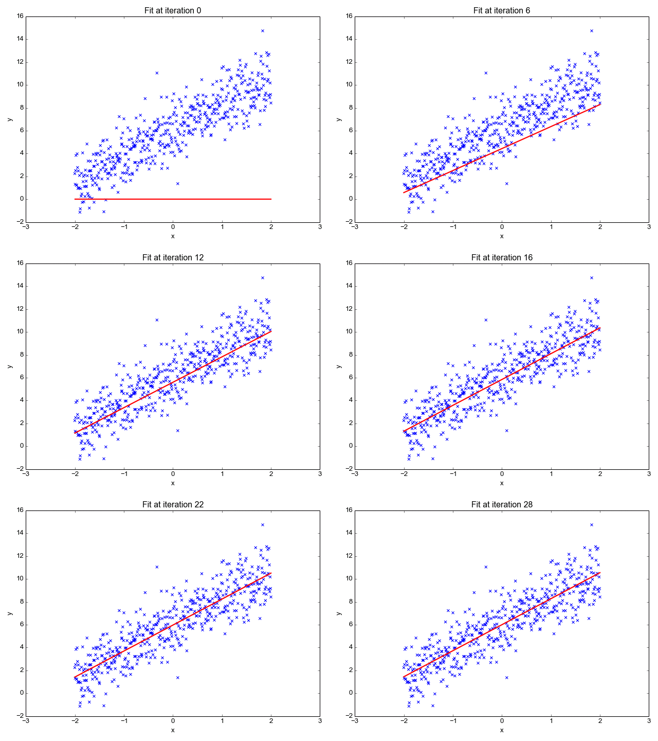
From “Linear Regression the Easier Way,” by Sagar Sharma.
Polynomial (Non-Linear) Regression
What happens when the relationship between our (single) variable age and output LOS is not linear?
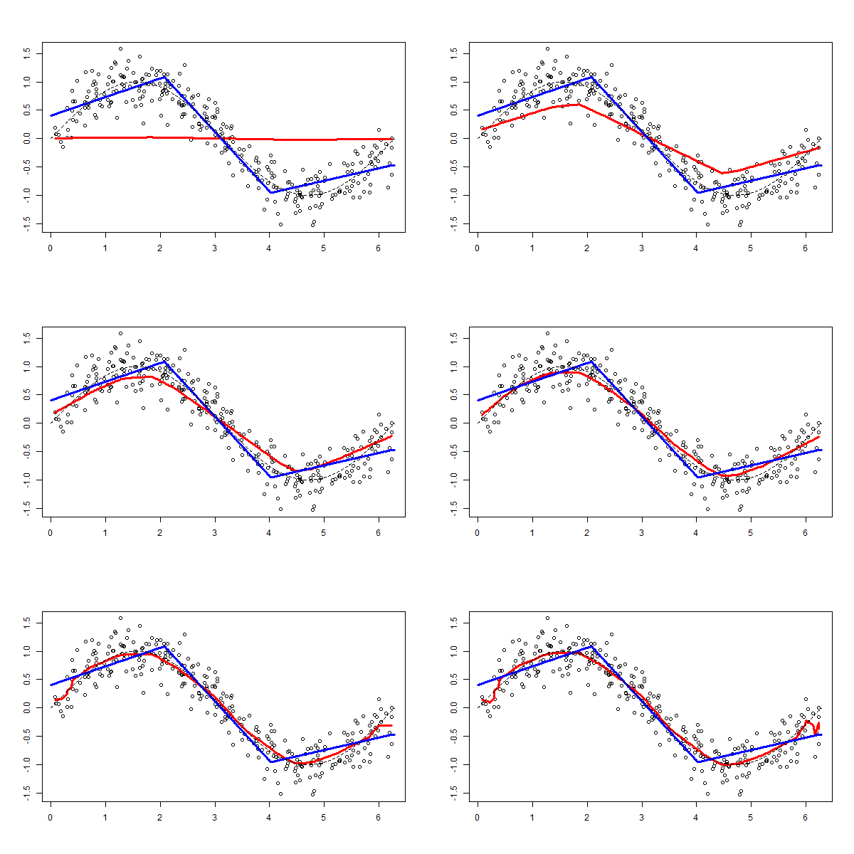
- The Task is to find the best line — obviously not a straight line — to describe the (non-linear) polynomial relationship between X (Age) and Y (LOS).
- Experience and Performance stay the same as in the previous example.
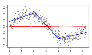
As above, monitoring the model learning process as it approximates the data (Experience) during the fit process:
From “R-english Freakonometrics” by Arthur Carpentier.
Life is a bit more complicated than one feature (age) when predicting LOS, so we’d like see what happens with two features — age and BMI. How do they contribute to LOS when taken together?
- The Task is to predict the Z axis (vertical) with a set of X and Y (horizontal plane).
- The Experience. The model now has two features: age and BMI. The output stays the same: LOS.
- Performance is measured as above.
Find the following peaks chart — a function — similar to the linear line or the polynomial line we found above.
This time the function defines the input as a plane (age on X and BMI on Y) and the output LOS on Z axis.
Knowing a specific age as X and BMI as Y and using such a function / peaks 3D chart, one can predict LOS as Z:
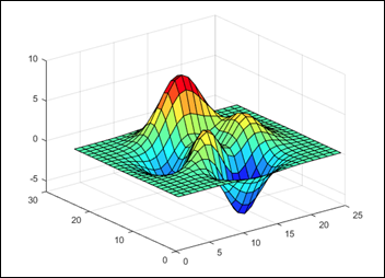
A peaks chart usually has a contour chart accompanying, visualizing the relationships between X, Y, and Z (note that besides X and Y, color is considered a dimension, too, Z on a contour chart). The contour chart of the 3D chart above:
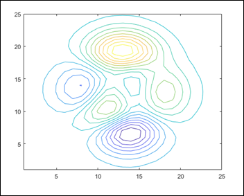
From the MathWorks manual.
How does a 4D problem look?
If we add the time as another dimension to a 3D like the one above, it becomes a 4D chart (disregard the axes and title):
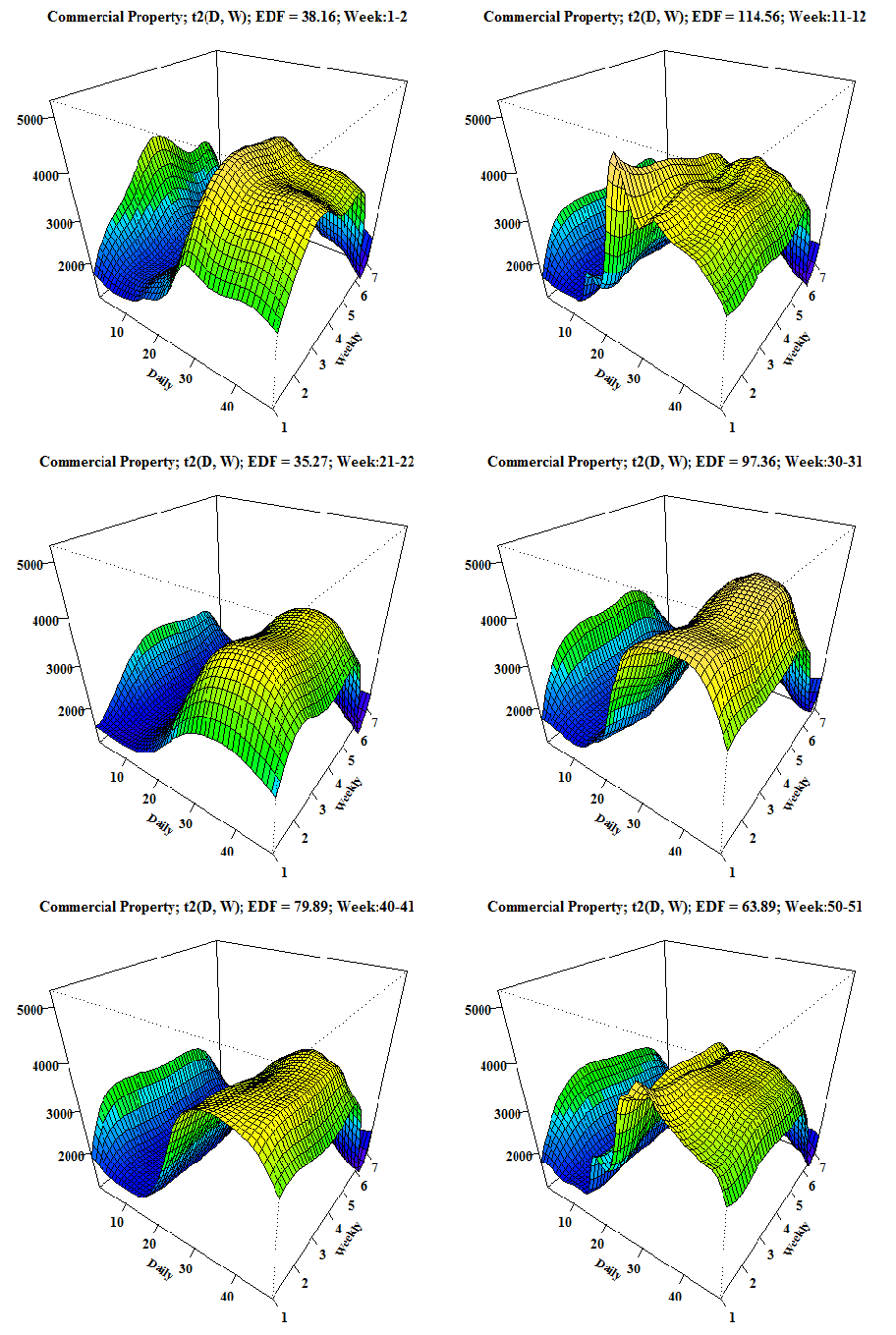
From “Doing Magic and Analyzing Time Series with R,” by Peter Laurinec.
Supervised Learning – Classification
When the output is discrete rather than continuous, the problem is one of classification.
Note: classification problems are also called logistic regression. That’s a misnomer and just causes confusion.
- Binary classification, such as dead or alive.
- Multi-class classification, such as discharged home, transferred to another facility, discharged to nursing facility, died, etc.
One can take a regression problem such as LOS and make it a classification problem using several buckets or classes: LOS between zero and four days, LOS between five and eight days, LOS greater than nine days, etc.
Binary Classification with Two Variables
- The Task is to find the best straight line that separates the blue and red dots, the decision boundary between the two classes.
- The Experience. Given the input of the X and Y coordinate of each dot, predict the output as the color of the dot — blue or red.
- Performance is the accuracy of the prediction. Note that just by chance, with no ML involved, the accuracy of guessing is expected to be around 50 percent in this of type of binary classification, as the blue and the red classes are well balanced.
In visualizing the data, it seems there may be a relatively straight line to separate the dots:
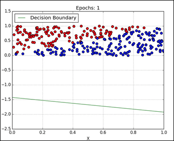
The model learning iteratively the best separating straight line. This model is linearly constrained when searching for a decision boundary:
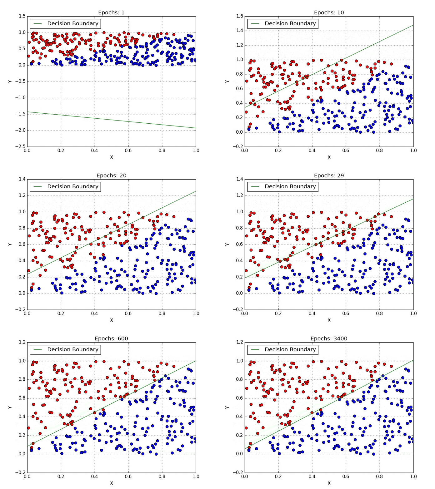
From “Classification” by Davi Frossard.
Binary Classification with a Non-Linear Separation
A bit more complex dots separation exercise, when the separation line is obviously non-linear.
The Task, Experience, and Performance remain the same:
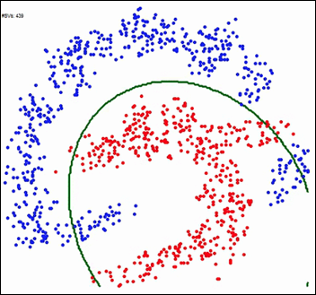
The ML model learning the best decision boundary, while not being constrained to a linear solution:
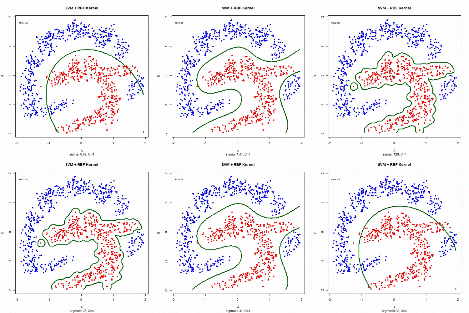
From gfycat.
Multi-Class Classification
Multi-class classification is actually an extension of the simple binary classification. It’s called the “One vs. All” technique.
Consider three groups: A, B, and C. If we know how to do a Binary classification (see above), then we can calculate probabilities for:
- A vs. all the others (B and C)
- B vs. all the others (A and C)
- C vs. all the others (A and B)
More about Classification models in the next articles.
Binary Classification with Three Variables
While the last example had two variables (X and Y) with one output (color of the dot), the next one has three input variables (X, Y, and Z) and the same output: color of the dot.
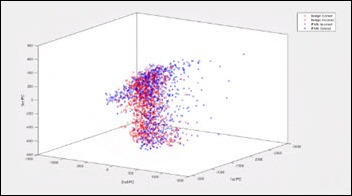
- The Task is to find the best hyperplane shape (also known as rules / function) to separate the blue and red dots.
- Experience has now three input variables (X, Y, and Z) and one output label (the dot color).
- Performance remains the same.
From Ammon Washburn, data scientist. Click here to see the animated 3D picture.
How can we visualize a problem with 5,000 dimensions?
Unfortunately, we cannot visualize more than 4-5 dimensions. The above 4D chart (3D plus time) on a map with multiple locations — charts running in parallel, over time — I guess that would be considered a 5D visualization, having the geo location as the fifth dimension. One can imagine how difficult it would be to actually visualize, absorb, and digest the information and just monitor such a (limited) 5D problem for a couple of days.
Alas, if it’s difficult for us to visualize and monitor a 5D problem, how can we expect to learn from each and every experience of such a complex system and improve our performance, in real time, on a prediction task?
How about a problem with 10,000 features, the task of predicting one out of 467 DRG classifications for a specific patient with an error less than 8 percent?
In this series, we’ll tackle problems with many features and many dimensions while visualizing additional monitors — the ML learning curves — which in my opinion are as beautiful and informative as the charts above, even as they are only 2D.
Other ML Architectures
On an artsy note, as it is related to the third group of ML models (Other) in my chart above, are models that are not purely supervised or unsupervised.
In 2015, Gatys et al. published a paper on a model that separates style from content in a painting. The generative model learns an artist’s style and then predicts the style effects learned on any arbitrary image. The left upper corner is an image in Europe and then each cell is the same image rendered in one of several famous painters’ styles:
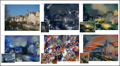
Scoff you may, but this week, the first piece of art generated by AI goes for sale at Christie’s.
Generative ML models have been trained to generate text in a Shakespearean style or the Bible style by feeding ML models with all Shakespeare or the whole Bible text. There are initiatives I’ll report about where a ML model learns the style of a physician or group of physicians and then creates admission / discharge notes accordingly. This is the ultimate dream come true for any young and tired physician or resident.
In Closing
I’d like to end this article on a philosophical note.
Humans recently started feeding ML models the actual Linux and Python programming languages (the relevant documentation, manuals, Q&A forums, etc.)
As expected, the machines started writing computer code on their own.
The computer software written by machines cannot be compiled nor executed and it will not actually run.
Yet …
I’ll leave you with this intriguing, philosophical, recursive thought in mind — computers writing their own software — until the next article in the series: Unsupervised Learning.


Apparently harder than this guy could code at least. I suspect the legal grey area is when they're offering a…